3D Oriented bounding boxes made simple
Calculating 3D oriented bounding boxes. Oriented boxes are useful to avoid obstacles and make best utilitsation of the real navigationable space for autonomous vehicles to steer around.


Overview
In the previous post we looked at the process of generating a 2D bounding box around some data/cluster of points. But while working with LIDARs i.e. point cloud data respectively, we would want the bounding boxes to be in 3-dimensions just like the data.
2D Oriented bounding boxes recap
As a quick recap, the steps involved in generating 2D oriented box is as follows-
- Translate the data to match the means to the origin
- Calculate the Eigen-vectors
- Find the inclination/orientation angle of the principal component i.e. the Eigen-vector with highes Eigen-value
- Use the angle calculated in step 3 to align the data/Eigen-vectors to the cartesian basis vectors
- Calculate the bounding box by determining the max, min values along each dimension
- Undo the rotation and translation to both data and bounding box coordinates
Notes on difference in procedure to 3D oriented bounding boxes
Here we notice that Eigen-vectors, translation, and rotation tasks play the main role. Calculating Eigen-vectors and performing translation is a straight forward task in 3D also but rotation is not. As, rotation around orthogonal axis is not commutative i.e. the order in which the layers of a Rubiks cube are rotated matters. That is changing the order in which the layers are rotated will result in a completely different colour patterns on the Rubiks cube. This non-commutative nature of rotations is shown below (feel free to skip to the next section if you are already aware of this)
%matplotlib widget
import matplotlib.pyplot as plt
import numpy as np
import numpy.linalg as LA
from mpl_toolkits.mplot3d import Axes3D
def yaw(theta):
    theta = np.deg2rad(theta)
    return np.array([[np.cos(theta), -np.sin(theta), 0],
                     [np.sin(theta),  np.cos(theta), 0],
                     [            0,              0, 1]])

def pitch(theta):
    theta = np.deg2rad(theta)
    return np.array([[np.cos(theta) , 0, np.sin(theta)],
                     [             0, 1,             0],
                     [-np.sin(theta), 0, np.cos(theta)]])

def roll(theta):
    theta = np.deg2rad(theta)
    return np.array([[1,              0,             0],
                     [0,  np.cos(theta), np.sin(theta)],
                     [0, -np.sin(theta), np.cos(theta)]])
def CreateFigure():
    """
    Helper function to create figures and label axes
    """
    fig = plt.figure()
    ax = fig.add_subplot(111, projection='3d')
    ax.set_xlabel('x')
    ax.set_ylabel('y')
    ax.set_zlabel('z')
    return ax
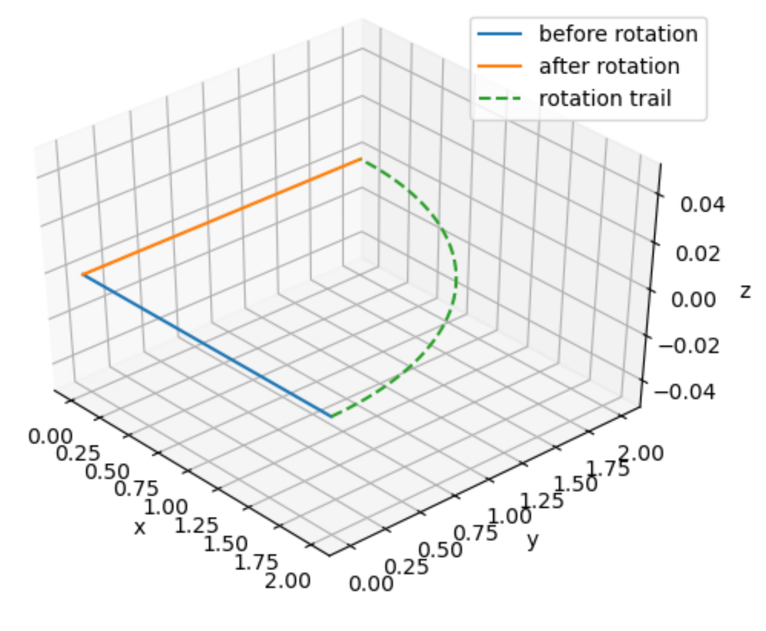
x = np.matmul(yaw(90), np.array([[2],
                                 [0],
                                 [0]]))
ax = CreateFigure()

ax.plot([0, 2], [0, 0], [0, 0], label="before rotation")
ax.plot([0, x[0,0]], [0, x[1,0]], [0, x[2,0]], label="after rotation")
ax.plot(2 * np.cos(np.linspace(0, np.pi/2, 50)), 2 * np.sin(np.linspace(0, np.pi/2, 50)), 0, linestyle="dashed", label="rotation trail")
ax.legend()
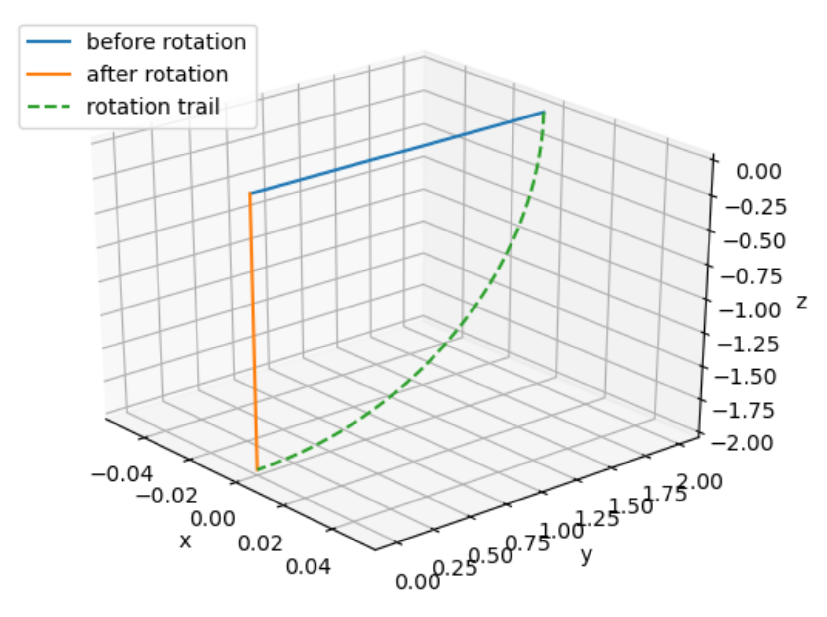
x = np.matmul(roll(90), np.array([[0],
                                  [2],
                                  [0]]))
ax = CreateFigure()

ax.plot([0, 0], [0, 2], [0, 0], label="before rotation")
ax.plot([0, x[0,0]], [0, x[1,0]], [0, x[2,0]], label="after rotation")
ax.plot(np.zeros(50), 2 * np.cos(np.linspace(0, np.pi/2, 50)), -2 * np.sin(np.linspace(0, np.pi/2, 50)), linestyle="dashed", label="rotation trail")
ax.legend()
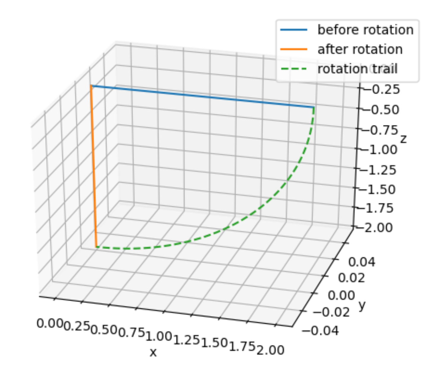
x = np.matmul(pitch(90), np.array([[2],
                                   [0],
                                   [0]]))
ax = CreateFigure()

ax.plot([0, 2], [0, 0], [0, 0], label="before rotation")
ax.plot([0, x[0,0]], [0, x[1,0]], [0, x[2,0]], label="after rotation")
ax.plot(2 * np.cos(np.linspace(0, np.pi/2, 50)), np.zeros(50), -2 * np.sin(np.linspace(0, np.pi/2, 50)), linestyle="dashed", label="rotation trail")
ax.legend()
basis = np.array([[1,0,0],
                  [0,1,0],
                  [0,0,1]])
x1 = np.matmul(yaw(90) @ pitch(90), np.array([[2], [0], [0]]))
x2 = np.matmul(pitch(90) @ yaw(90), np.array([[2], [0], [0]]))
def SetAxisProp(ax):
    ax.set_xlabel('x')
    ax.set_ylabel('y')
    ax.set_zlabel('z')
    ax.set_xlim(-2, 2)
    ax.set_ylim(-2, 2)
    ax.set_zlim(-2, 2)

fig = plt.figure(figsize=(10,6))
ax1 = fig.add_subplot(121, projection='3d')
SetAxisProp(ax1)
ax2 = fig.add_subplot(122, projection='3d')
SetAxisProp(ax2)

ax1.set_title("Yaw x Pitch")
ax1.plot([0, 2], [0, 0], [0, 0], label="before rotation")
ax1.plot([0, x1[0,0]], [0, x1[1,0]], [0, x1[2,0]], label="after rotation")
ax1.legend()

ax2.set_title("Pitch x Yaw")
ax2.plot([0, 2], [0, 0], [0, 0], label="before rotation")
ax2.plot([0, x2[0,0]], [0, x2[1,0]], [0, x2[2,0]], label="after rotation")
ax2.legend()
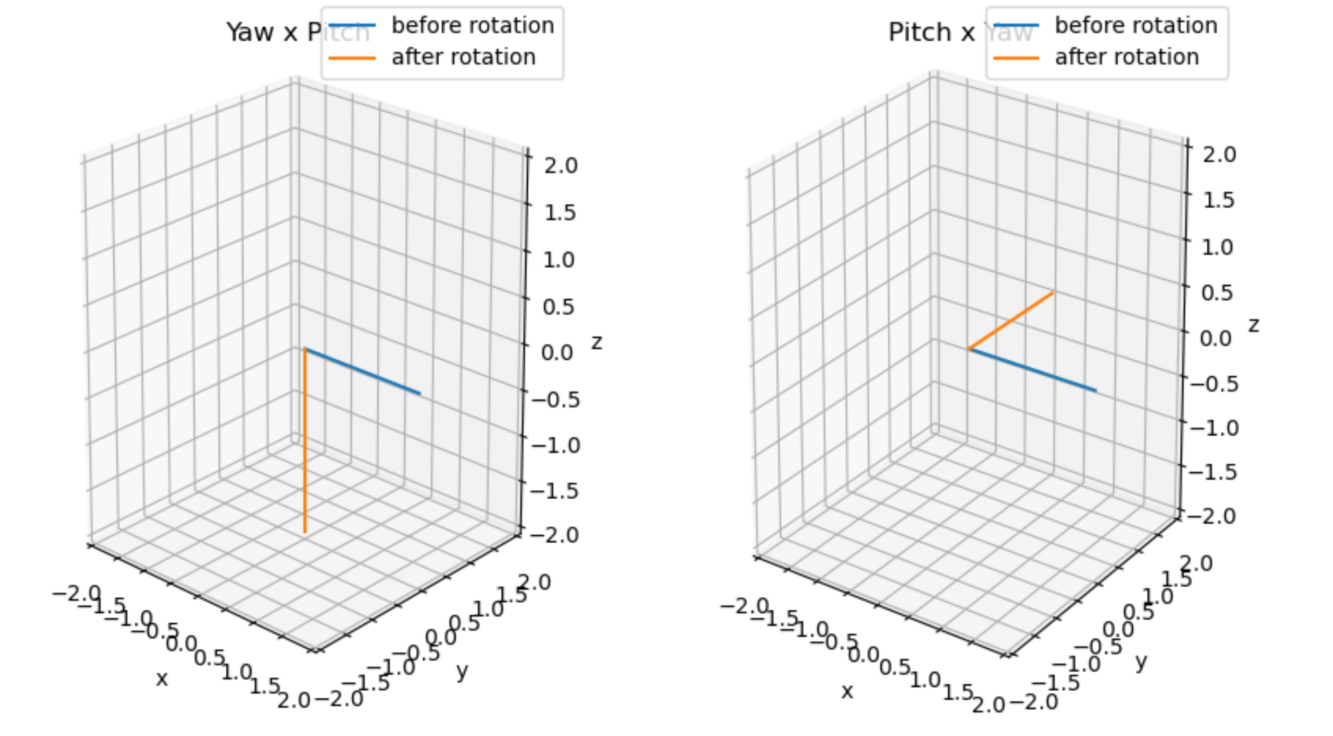
As we can see in the figure above, just changing the order in which yaw and pitch the vector, the resulting vector is completely different!
So, in this post the main difference compared to the previous post involving 2D oriented bounding boxes would be concerned with rotation and the way we align the data to the cartesian basis.
A quick overiew of what is to come
Let us get started with the code and the math to generate a bounding box
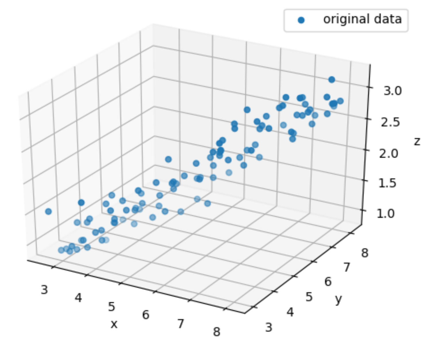
x = np.linspace(3, 8, 100) + np.random.normal(0, 0.2, 100)
y = np.linspace(3, 8, 100) + np.random.normal(0, 0.2, 100)
z = np.linspace(1, 3, 100) + np.random.normal(0, 0.2, 100)
data = np.vstack([x, y, z])

fig = plt.figure()
ax = fig.add_subplot(111, projection='3d')
ax.scatter(data[0,:], data[1,:], data[2,:], label="original data")
ax.set_xlabel('x')
ax.set_ylabel('y')
ax.set_zlabel('z')
ax.legend()
means = np.mean(data, axis=1)
cov = np.cov(data)
eval, evec = LA.eig(cov)
eval, evec
np.rad2deg(np.arccos(np.dot(evec[:,0], evec[:,1])))
np.rad2deg(np.arccos(np.dot(evec[:,1], evec[:,2])))
np.rad2deg(np.arccos(np.dot(evec[:,2], evec[:,0])))
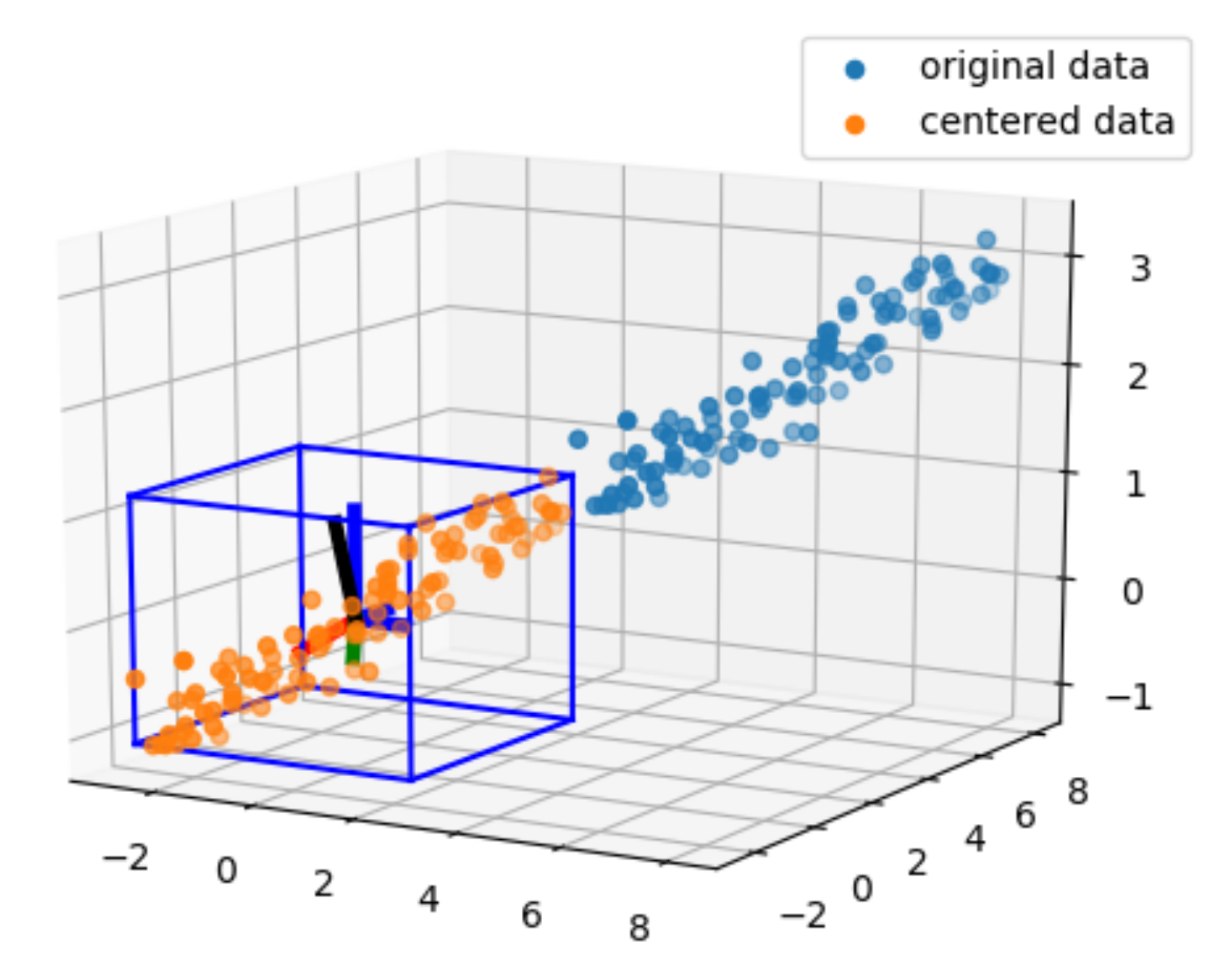
centered_data = data - means[:,np.newaxis]
fig = plt.figure()
ax = fig.add_subplot(111, projection='3d')
ax.scatter(data[0,:], data[1,:], data[2,:], label="original data")
ax.scatter(centered_data[0,:], centered_data[1,:], centered_data[2,:], label="centered data")
ax.legend()
# cartesian basis
ax.plot([0, 1],  [0, 0], [0, 0], color='b', linewidth=4)
ax.plot([0, 0],  [0, 1], [0, 0], color='b', linewidth=4)
ax.plot([0, 0],  [0, 0], [0, 1], color='b', linewidth=4)
# eigen basis
ax.plot([0, evec[0, 0]],  [0, evec[1, 0]], [0, evec[2, 0]], color='r', linewidth=4)
ax.plot([0, evec[0, 1]],  [0, evec[1, 1]], [0, evec[2, 1]], color='g', linewidth=4)
ax.plot([0, evec[0, 2]],  [0, evec[1, 2]], [0, evec[2, 2]], color='k', linewidth=4)
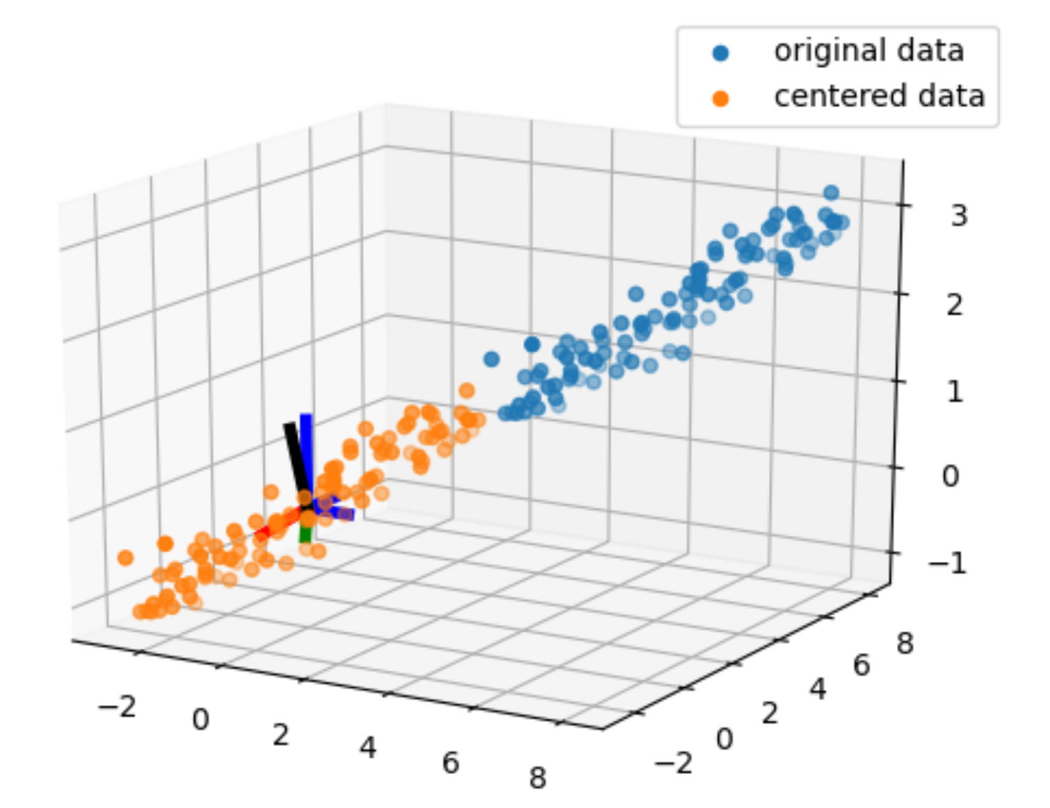
The axis orthogonal axes in blue are the cartesian basis and the ones in red, green, and black are the orthogonal eigen vector
def draw3DRectangle(ax, x1, y1, z1, x2, y2, z2):
    # the Translate the datatwo sets of coordinates form the apposite diagonal points of a cuboid
    ax.plot([x1, x2], [y1, y1], [z1, z1], color='b') # | (up)
    ax.plot([x2, x2], [y1, y2], [z1, z1], color='b') # -->
    ax.plot([x2, x1], [y2, y2], [z1, z1], color='b') # | (down)
    ax.plot([x1, x1], [y2, y1], [z1, z1], color='b') # <--

    ax.plot([x1, x2], [y1, y1], [z2, z2], color='b') # | (up)
    ax.plot([x2, x2], [y1, y2], [z2, z2], color='b') # -->
    ax.plot([x2, x1], [y2, y2], [z2, z2], color='b') # | (down)
    ax.plot([x1, x1], [y2, y1], [z2, z2], color='b') # <--

    ax.plot([x1, x1], [y1, y1], [z1, z2], color='b') # | (up)
    ax.plot([x2, x2], [y2, y2], [z1, z2], color='b') # -->
    ax.plot([x1, x1], [y2, y2], [z1, z2], color='b') # | (down)
    ax.plot([x2, x2], [y1, y1], [z1, z2], color='b') # <--
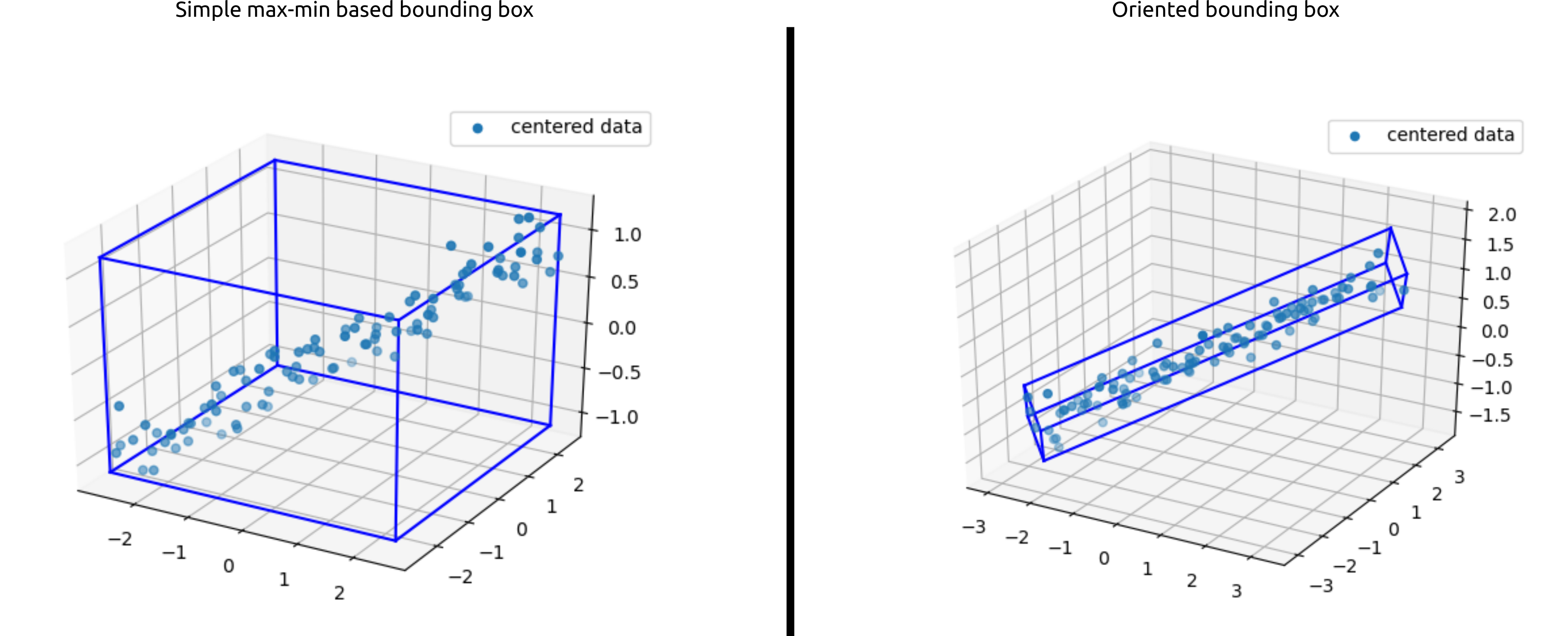
xmin, xmax, ymin, ymax, zmin, zmax = np.min(centered_data[0, :]), np.max(centered_data[0, :]), np.min(centered_data[1, :]), np.max(centered_data[1, :]), np.min(centered_data[2, :]), np.max(centered_data[2, :])
# Code repeat start
fig = plt.figure()
ax = fig.add_subplot(111, projection='3d')
ax.scatter(data[0,:], data[1,:], data[2,:], label="original data")
ax.scatter(centered_data[0,:], centered_data[1,:], centered_data[2,:], label="centered data")
ax.legend()
# cartesian basis
ax.plot([0, 1],  [0, 0], [0, 0], color='b', linewidth=4)
ax.plot([0, 0],  [0, 1], [0, 0], color='b', linewidth=4)
ax.plot([0, 0],  [0, 0], [0, 1], color='b', linewidth=4)
# eigen basis
ax.plot([0, evec[0, 0]],  [0, evec[1, 0]], [0, evec[2, 0]], color='r', linewidth=4)
ax.plot([0, evec[0, 1]],  [0, evec[1, 1]], [0, evec[2, 1]], color='g', linewidth=4)
ax.plot([0, evec[0, 2]],  [0, evec[1, 2]], [0, evec[2, 2]], color='k', linewidth=4)
# Code repeat end
draw3DRectangle(ax, xmin, ymin, zmin, xmax, ymax, zmax)
Rotation! the crux of the process in generating the oriented bounding box
As previously mentioned that the Eigen-vectors are pre normalised and that they are orthogonal to each other when we checked the angles between them, in effect we have in our hands a new set of basis vectors. We can use this basis vector to transform coordinates to and fro defined using any other basis vectors.
That is, in our case the Eigen-vectors matrix evec can be used to transform coordinates defined in the basis vectors (1,0,0), (0,1,0), (0,0,1). Let us denote the coordinates in the cartesian basis vectors as C and the coordinates with Eigen-vectors as basis as E.
- We can transform coordinated from C to E by multiplying with the evec basis vector matrix
- We can transform coordinated from E to C by multiplying with the inverse(evec) basis vector matrix
Since the Eigen-vectors are normalised, the inverse(evec) == transpose(evec) (the code below proves this)
np.allclose(LA.inv(evec), evec.T)
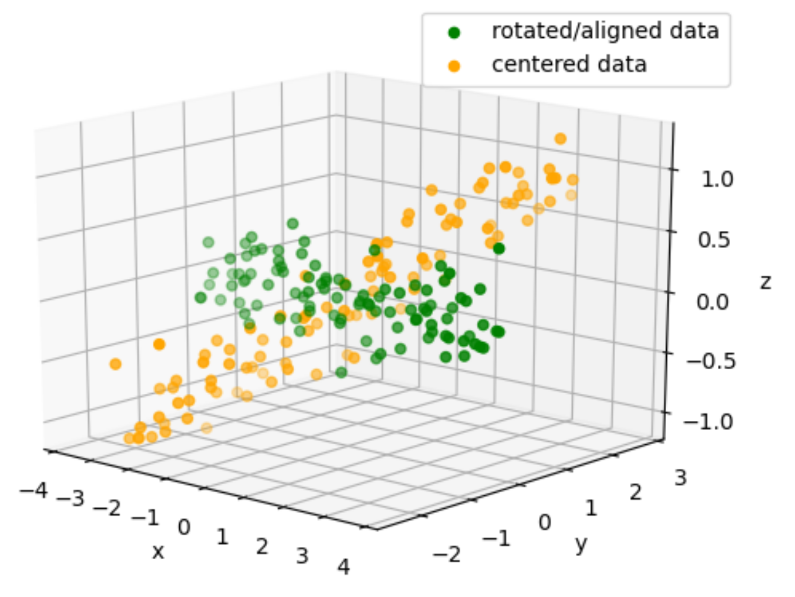
aligned_coords = np.matmul(evec.T, centered_data)
fig = plt.figure()
ax = fig.add_subplot(111, projection='3d')
ax.scatter(aligned_coords[0,:], aligned_coords[1,:], aligned_coords[2,:], color='g', label="rotated/aligned data")
ax.scatter(centered_data[0,:], centered_data[1,:], centered_data[2,:], color='orange', label="centered data")
ax.legend()
ax.set_xlabel('x')
ax.set_ylabel('y')
ax.set_zlabel('z')
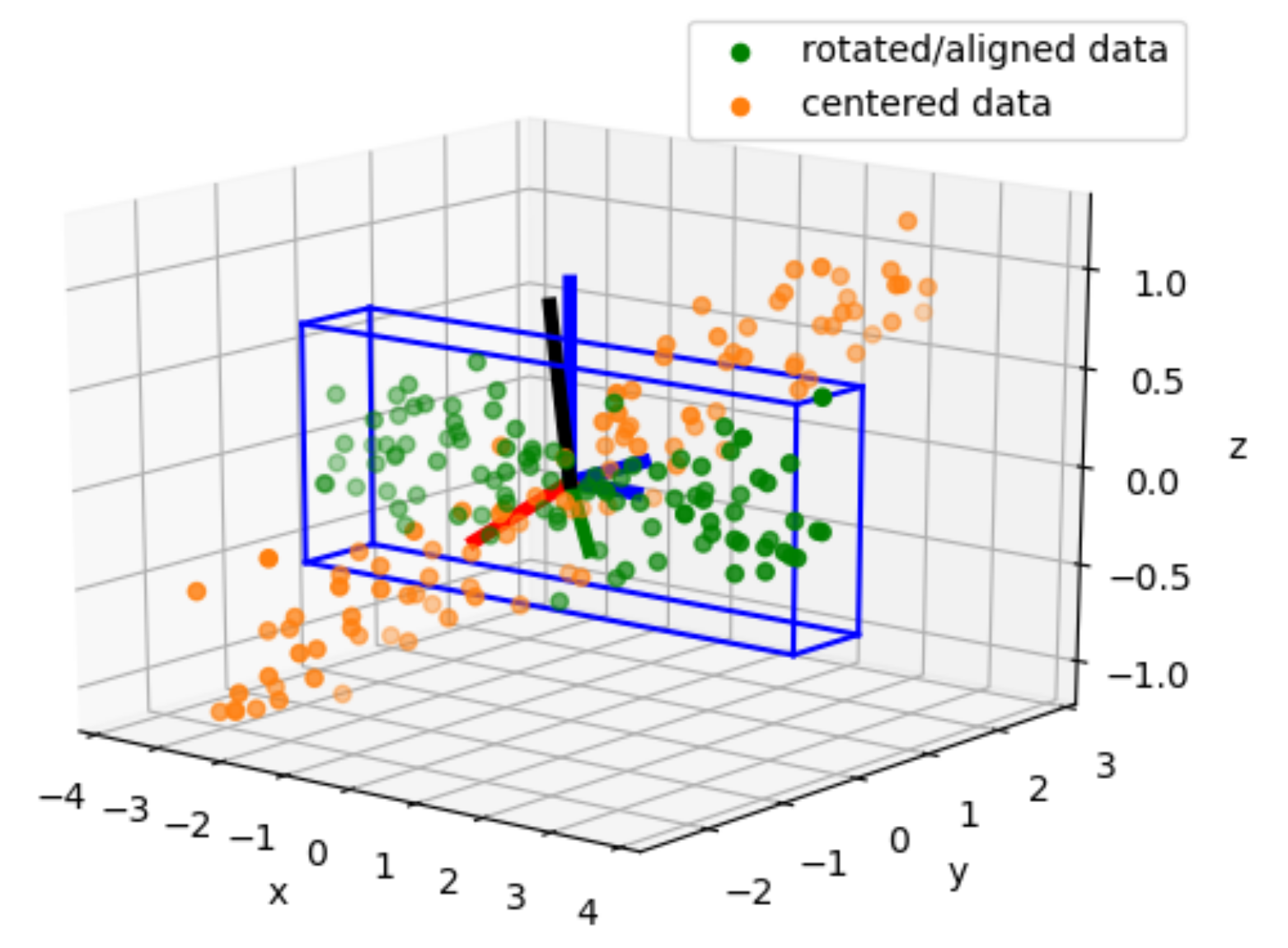
xmin, xmax, ymin, ymax, zmin, zmax = np.min(aligned_coords[0, :]), np.max(aligned_coords[0, :]), np.min(aligned_coords[1, :]), np.max(aligned_coords[1, :]), np.min(aligned_coords[2, :]), np.max(aligned_coords[2, :])

fig = plt.figure()
ax = fig.add_subplot(111, projection='3d')
ax.scatter(aligned_coords[0,:], aligned_coords[1,:], aligned_coords[2,:], color='g', label="rotated/aligned data")
ax.scatter(centered_data[0,:], centered_data[1,:], centered_data[2,:], color='tab:orange', label="centered data")
ax.legend()
ax.set_xlabel('x')
ax.set_ylabel('y')
ax.set_zlabel('z')
# cartesian basis
ax.plot([0, 1],  [0, 0], [0, 0], color='b', linewidth=4)
ax.plot([0, 0],  [0, 1], [0, 0], color='b', linewidth=4)
ax.plot([0, 0],  [0, 0], [0, 1], color='b', linewidth=4)
# eigen basis
ax.plot([0, evec[0, 0]],  [0, evec[1, 0]], [0, evec[2, 0]], color='r', linewidth=4)
ax.plot([0, evec[0, 1]],  [0, evec[1, 1]], [0, evec[2, 1]], color='g', linewidth=4)
ax.plot([0, evec[0, 2]],  [0, evec[1, 2]], [0, evec[2, 2]], color='k', linewidth=4)

draw3DRectangle(ax, xmin, ymin, zmin, xmax, ymax, zmax)
rectCoords = lambda x1, y1, z1, x2, y2, z2: np.array([[x1, x1, x2, x2, x1, x1, x2, x2],
                                                      [y1, y2, y2, y1, y1, y2, y2, y1],
                                                      [z1, z1, z1, z1, z2, z2, z2, z2]])

realigned_coords = np.matmul(evec, aligned_coords)
realigned_coords += means[:, np.newaxis]

rrc = np.matmul(evec, rectCoords(xmin, ymin, zmin, xmax, ymax, zmax))
# rrc = rotated rectangle coordinates
rrc += means[:, np.newaxis]
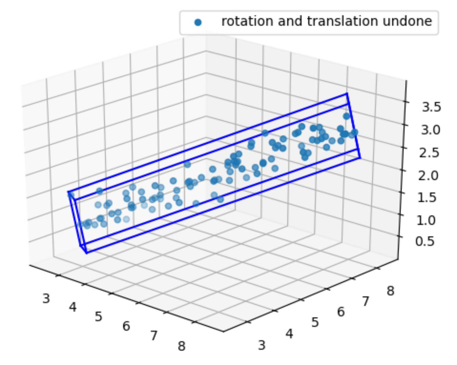
fig = plt.figure()
ax = fig.add_subplot(111, projection='3d')
ax.scatter(realigned_coords[0,:], realigned_coords[1,:], realigned_coords[2,:], label="rotation and translation undone")
ax.legend()

# z1 plane boundary
ax.plot(rrc[0, 0:2], rrc[1, 0:2], rrc[2, 0:2], color='b')
ax.plot(rrc[0, 1:3], rrc[1, 1:3], rrc[2, 1:3], color='b')
ax.plot(rrc[0, 2:4], rrc[1, 2:4], rrc[2, 2:4], color='b')
ax.plot(rrc[0, [3,0]], rrc[1, [3,0]], rrc[2, [3,0]], color='b')

# z2 plane boundary
ax.plot(rrc[0, 4:6], rrc[1, 4:6], rrc[2, 4:6], color='b')
ax.plot(rrc[0, 5:7], rrc[1, 5:7], rrc[2, 5:7], color='b')
ax.plot(rrc[0, 6:], rrc[1, 6:], rrc[2, 6:], color='b')
ax.plot(rrc[0, [7, 4]], rrc[1, [7, 4]], rrc[2, [7, 4]], color='b')

# z1 and z2 connecting boundaries
ax.plot(rrc[0, [0, 4]], rrc[1, [0, 4]], rrc[2, [0, 4]], color='b')
ax.plot(rrc[0, [1, 5]], rrc[1, [1, 5]], rrc[2, [1, 5]], color='b')
ax.plot(rrc[0, [2, 6]], rrc[1, [2, 6]], rrc[2, [2, 6]], color='b')
ax.plot(rrc[0, [3, 7]], rrc[1, [3, 7]], rrc[2, [3, 7]], color='b')