Gaussian Matrix
Generating a Gaussian matrix for applying Gaussian Blur to an Image


Overview
In image processing, a Gaussian blur (also known as Gaussian smoothing) is the result of blurring an image by a Gaussian function (named after mathematician and scientist Carl Friedrich Gauss).
It is a widely used effect in graphics software, typically to reduce image noise and reduce detail. The visual effect of this blurring technique is a smooth blur resembling that of viewing the image through a translucent screen.
Gaussian smoothing is also used as a pre-processing stage in computer vision algorithms in order to enhance image structures at different scales—see scale space representation and scale space implementation.(Wikipedia contributors, 2021)
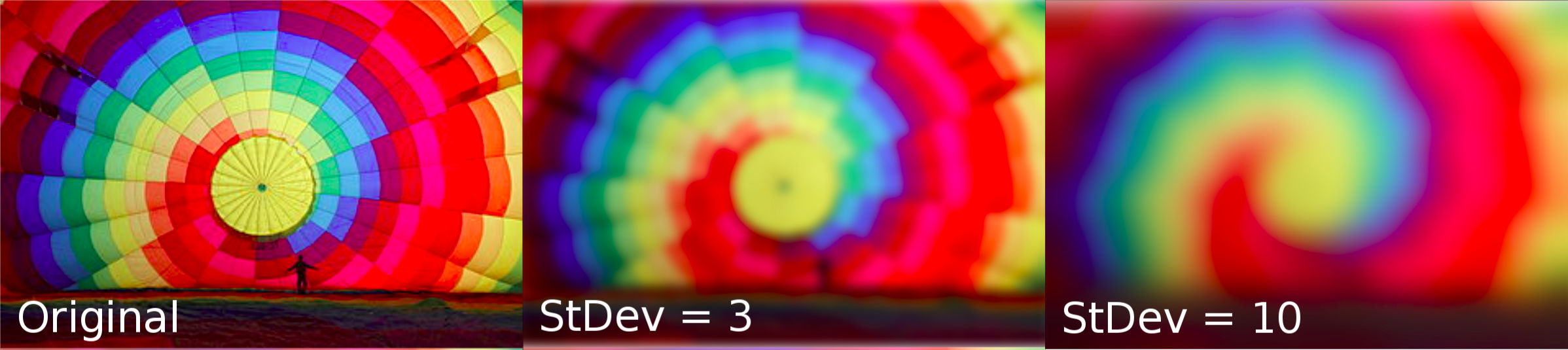
The following is an example showing an unblurred image along with two levels of blurrings applied.
What to expect?
In this article we will see how to create one such kernel/matrix which has it's entries in agreement with a Gaussian distribution. Using the generated matrix to convolve and produce a blurred version of a image is not covered in this article as this is a very common operation which is available in numpy, scipy and more.
Some basics
The general form of its probability density function is, ${\displaystyle f(x)={\frac {1}{\sigma {\sqrt {2\pi }}}}e^{-{\frac {1}{2}}\left({\frac {x-\mu }{\sigma }}\right)^{2}}}$
Now, we know the kind of distribution we need and we also have the necessary formula but what we need is an apporpriate way to place the entries in a $N x N$ matrix (where N is odd) with the entries values radially decreasing in all directions.
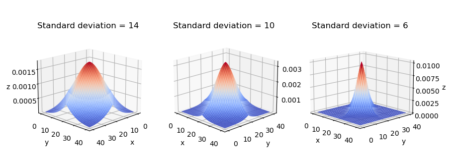
When a 3D graph of the matrix entries is drawn using the information of entries positions in the matrix and their values, the resulting 3D graph should resembel a 3D Normal distribution curve. Which we will see at the end of this article.
Main solution Idea
The general solution to the problem of correctly mapping the matrix locations to their respective likelihoods can be solved by noting that the resulting 3D Normal distribution graph will be symmetric in nature and an odd sized matrix has unique center element.
In the code below, we breakdown an odd sized matrix into 4 quadrants and utilise the top left quadrant to generate the matrix entries. In the above formula, we will replace $x$ with (row No.+ column No.) i.e., ${\displaystyle f(R+C)={\frac {1}{\sigma {\sqrt {2\pi }}}}e^{-{\frac {1}{2}}\left({\frac {(R+C)-\mu }{\sigma }}\right)^{2}}}$ where-
- R - Row Number
- C - Column Number
%matplotlib widget
import numpy as np
from matplotlib import cm
import matplotlib.pyplot as plt
from mpl_toolkits.mplot3d import Axes3D
def GM(std_dev, size):
    """
    Computes a gaussian matrix/kernel of given size
    :param std_dev: Standard deviation of the Gaussian
    :param size: Size of kernel needed
    """
    if (size % 2 != 1):
        print("Size has to be odd")
        return
    # Gaussian parameters and normalizing constant
    sigma = std_dev
    # Variance
    var = sigma **2
    # Normalisation parameter (is constant for all matrix entries)
    norm = 1/(np.sqrt(2*np.pi)*sigma)

    def density(x):
        return norm * np.exp(-0.5*(x)**2/var)

    # quarter kernel size
    qs = (size//2) + 1
    # quarter kernel
    qk = np.zeros((qs, qs))
    for R in range(qs):
        for C in range(qs):
            qk[R,C] = density(2*qs - (R+C))
    # mirror the kernel verticaly and horizontaly
    kernel = np.hstack((qk, np.flip(qk,1)[:,1:]))
    kernel = np.vstack((kernel, np.flip(kernel,0)[1:,:]))
    # normalise the weights
    kernel = kernel / np.sum(kernel)

    return kernel
kernel_size = 41
idxs = np.indices((kernel_size, kernel_size))
fig = plt.figure(figsize=(10,4))
std_devs = [14, 10, 6]
for i, std in enumerate(std_devs):
    fig_idx = 100 + len(std_devs)*10 + 1 + i
    gaussiann_kernel = GM(std, kernel_size)
    ax = fig.add_subplot(fig_idx, projection='3d')
    # ax.scatter(idxs[0].reshape(-1), idxs[1].reshape(-1), gaussiann_kernel.reshape(-1))
    ax.plot_surface(idxs[0], idxs[1], gaussiann_kernel, cmap=cm.coolwarm)
    ax.set_title(f"Standard deviation = {std}")
    ax.set_xlabel('x')
    ax.set_ylabel('y')
    ax.set_zlabel('z')